Analysing power consumption in cellular IoT systems
The Internet of Things (IoT) covers a wide range of devices, ranging in size, dedicated to a particular task and increasingly found everywhere. They can be divided into three main categories based on their application – consumer, enterprise and industrial.
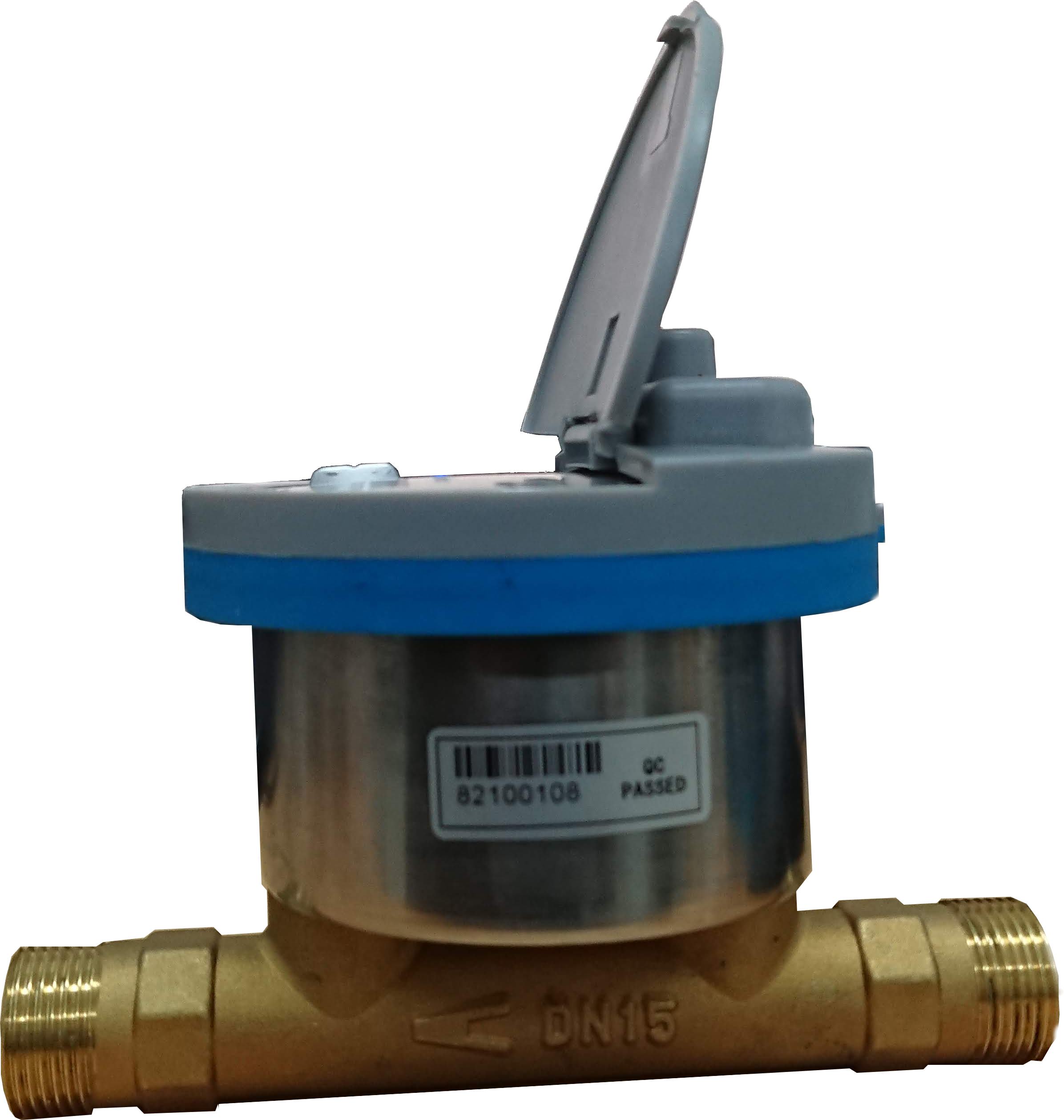
The consumer oriented IoT devices are widely known – smart TVs, smart speakers, wearables, toys and many more enhance our daily lives and bring us entertainment. On the other hand, there are devices such as smart meters, traffic/weather monitors, smart thermostats, smart lights and others which make our life more comfortable and reduce costs by helping us make better use of energy. These kinds of devices are driven by enterprises and industry.
One key factor in IoT is the power consumption of the devices themselves. This is even more true with the enterprise and industrial categories. An IoT device may be installed at a site to carry out work for many years to come and is often equipped with a battery which cannot be replaced. This means that the end of the battery’s life also means the end of the device’s life. With a device’s lifetime reaching up to 10 or more years, particularly in the case of 5G mobile networks, engineers need to make sure a battery can last in the field for as long as possible.
However, 5G networks are still not widely deployed, being more commonly used as private industry test networks. Most of the cellular IoT devices today still operate on the previous cellular generation, namely LTE technology.
With LTE, we have two options – the LPWAN (Low-Power Wide-Area Network) standard based on LTE is known as NB-IoT (Narrowband Internet of Things). This standard focuses on indoor coverage with its often-high network density. The emphasis is also on a long battery life for devices.
Next: IoT standards
The second popular standard is called LTE-M (specifically LTE Cat-M1) which addresses the need for machine-to-machine and IoT applications. It offers comparatively higher data rates and supports voice over the network but it costs more and is usually bandwidth hungry.
Support for these widely used standards is provided by tst systems such as the MT8821C Radio Communication Analyzer. The instrument supports Cat-M1 and both NB-IoT versions, NB-1 and NB-2. However, the machine is not designed to test only LPWAN technologies – it can also simulate other network technologies, such as LTE/Advanced, GSM, W-CDMA and more.
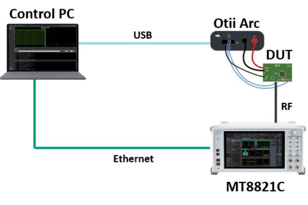
If we want to measure the power consumption of a device in a closed, controlled environment, using a standalone network simulator is not enough. We also need to measure power consumed by a device. This can be achieved by supplying power to a device using a SMU (Source Measuring Unit). The chosen SMU in our case is the Otii arc made by Swedish company Qoitech.
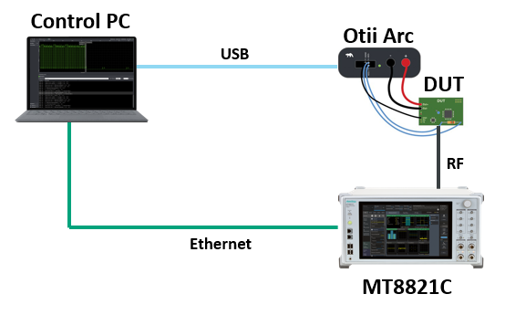

The test set-up includes a PC to control both instruments. The network simulator is connected to the PC via the Ethernet cable, allowing us to control the instrument remotely. The SMU’s server runs locally on the PC, which connects to the SMU via the USB cable. This makes possible a simple automation of the measurement.
The Otii arc comes with a GUI application which offers multiple possibilities. However, we will use only its graphical capability to show the energy consumed. During a measurement, the energy consumption is shown in real time. It can be recorded and processed later as needed.
Both instruments can be Python automated. To control the network simulator, the PyVisa module needs to be installed on the PC, in addition to Python itself. It provides the PC with all the necessary tools to communicate with the instrument using VISA (Virtual Instrument Software Architecture) commands and queries.
Communication and control for the Otii arc is provided by an API library offering a large number of functionalities. Even more important is that most of the frequent steps used in the GUI application can be replicated using pure Python. The preferred version of Python is version 3.7.
Next: Python script
Once the Python control script is ready, it can be verified. It is important to have all the equipment actively connected to the PC – a running Otii server and a running IP connection between the PC and the MT8821C instrument. Another necessity is a dictionary for translating codenames. Our main goal here is to import a signaling trace from the Anritsu instrument to the Otii GUI application. To do this, we need to translate a code number into a human readable text every time we receive a response from a sent query. Thanks to this implementation, we can see the power consumption at different stages of a radio communication.
Probably the hardest process to implement is a time synchronization of the instruments. The control PC, the Otii arc record and the MT8821C signaling trace’s timestamp all use different formats. Because of their nature we can theoretically go as low as 1ms, the lowest time resolution of the signaling trace. However, this measurement precision cannot be achieved in practice as there are delays due to the network communication and the executed processes.
The upper limit of precision is empirically obtained by multiple observations using protocol analyzer and other tests performed in Python. Once the time is adjusted based on these steps, we get the minimal guaranteed precision of +/- 250ms. It is important to note that the real precision is better than the guaranteed one. Often the true value is anywhere between 100-200ms, which can always be optimized further.
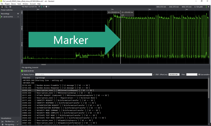
Once the signaling trace is imported and the time offset between the record and the signaling trace’s timestamp is adjusted, the result looks very promising. We can see different stages of the radio communication inside the GUI application. If we are interested in power consumption at the instant a DUT (Device Under Test) joins the network, we can see this easily by clicking on the imported trace line. It automatically shifts the power consumption graph and we can clearly see the energy level at the time thanks to the marker.

In this case, a DUT is continually supplied with a constant voltage power by the SMU, which may not be the case for the real world IoT device’s energy consumption. As mentioned earlier, IoT devices are usually equipped with batteries which are unable to hold a constant voltage over the lifetime of the device. To enhance the fidelity of the measurement, it is possible to simulate different types of batteries. The SMU can simulate different batteries’ power profiles, ranging from commercial batteries to those of our own design.
This solution is an excellent way to measure power consumption of an IoT device while verifying its network capabilities. It is important to know what the battery drainage is during different radio communication states.
The biggest impact on a battery is the peak performance of a device and the power saving mode (PSM) in which an IoT device is most often placed. The MT8821C instrument provides a test environment with perfected conditions where we can control the network parameters. Altogether, the set up provides a very scalable solution which can be used to monitor energy consumption of a specific network state and/or to benchmark different IoT devices.
 If you enjoyed this article, you will like the following ones: don't miss them by subscribing to :